Thursday 16 November 2017

Teaching to machines: What is learning in machine learning entails?

Preamble

Ebbinghaus (Wikipedia


Machine Learning (ML)
 is now a de-facto skill for every quantitative job and almost every industry embraced it, even though fundamentals of the field is not new at all. However, what does it mean to teach to a machine? Unfortunately, for even moderate technical people coming from different backgrounds, answer to this question is not apparent in the first instance. This sounds like a conceptual and jargon issue, but it lies in the very success of supervised learning algorithms.

What is a machine in machine learning

First of all here, machine does not mean a machine in conventional sense, but computational modules or set of instructions. It is called machine because of thermodynamics can be applied to analyse this computational modules, their algorithmic complexity can be map to an energy consumption and work production, recall Landauer Principle. Charles Bennett has an article on this principle, here.

Learning curve for machines

What about learning bit? Learning is a natural process for humans, specially for the younger ones. We learn new things naturally without explicitly thinking with instruction and some training, such as practised in University of Bologna a millennia ago. Usually,  it takes time for us to learn new thing, and the process is called learning curve, due to Hermann Ebinghauss. Essentially, learning in machine learning exactly roots in Ebinghauss approach.  But question remains, how this manifests quantitatively in machine learning. Answer to this question is going to be given here.

The concept of learning curve and  effect of sample size in training machine learning models for both experienced and novice practitioners. It is often this type of analysis is omitted in producing supervised learning solutions. In the advent of deep learning architecture, multi-layered neural networks, this concept becomes more pronounced.

Quantifying learning curve lies in measuring performance over increasing experience. If the performance of the machine, or human, increases over experience we denote that learning is achieved. We distinguish good learner.

On the misconception of unsupervised learning


Figure 2: Donald Webb,
father of unsupervised
learning.
(Source: Wikipedia)
A generic misconception appear on what unsupervised learning means. Clustering, or categorising unlabelled data, is not learning in Ebbinghaus sense. The goodness of fit or cluster validation exercise do not account an increase in experience, at least this is not established in the literature, judging from cluster validation techniques, see, Jain-Dubes's Algorithms for clustering data. Wikipedia defines unsupervised learning "inferring a function to describe hidden structure from "unlabeled" data", this is a function inference is not learning,.

Then, what is unsupervised learning? It originates from Hebbian Theory from neuroscience that "Cells that fire together wire together". This implies, unsupervised learning is about how information is encoded, not how it is labelled. One good practical model that could be classified as unsupervised learning, so called spiking network model.

Outlook

The concept of learning from Machine Learning perspective is summarised in this post. In data science, it is a good practice to differentiate what we call learning and function inference/optimisation. Being attentive to this details would help us.


Wednesday 16 August 2017

Understanding overfitting: an inaccurate meme in supervised learning

Kindly reposted to KDnuggets by Gregory Piatetsky-Shapiro with the title Understanding overfitting: an inaccurate meme in machine learning

Preamble There is a lot of confusion among practitioners regarding the concept of overfitting. It seems like, a kind of an urban legend or a meme, a folklore is circulating in data science or allied fields with the following statement:
Applying cross-validation prevents overfitting and a good out-of-sample performance, low generalisation error in unseen data, indicates not an overfit.

This statement is of course not true: cross-validation does not prevent your model to overfit and good out-of-sample performance does not guarantee not-overfitted model. What actually people refer to in one aspect of this statement is called overtraining. Unfortunately, this meme is not only propagated in industry but in some academic papers as well. This might be at best a confusion on jargon. But, it will be a good practice if we set the jargon right and clear on what do we refer to when we say overfitting, in communicating our results.

Aim In this post, we will give an intuition on why model validation as approximating generalization error of a model fit and detection of overfitting can not be resolved simultaneously on a single model. We will work on  a concrete example workflow in understanding overfitting, overtraining and a typical final model building stage  after some conceptual introduction. We will avoid giving a reference to the Bayesian interpretations and regularisation and restrict the post to regression and cross-validation. While regularisation has different ramification due to its mathematical properties and prior distributions have different implications in Bayesian statistics. We assume an introductory background in machine learning, so this is not a beginners tutorial.

A recent question from Andrew Gelman, a Bayesian guru, regarding What is overfitting? was one of the reasons why this post is developed along with my frustration to see practitioners being muddy on the meaning of overfitting and continuing recently published data science related technical articles circulating around and even in some academic papers claiming the above statement.

What do we need to satisfy in supervised learning? One of the most basic tasks in mathematics is to find a solution to a function: If we restrict ourselves to real numbers in $n$-dimensions and our domain of interest would be $\mathbb{R}^{n}$. Now imagine set of $p$ points living in this domain  $x_{i}$ form a dataset, this is actually a partial solution to a function. The main purpose of modelling is to find an explanation of the dataset, meaning that we need to determine $m$-parameters, $a \in \mathbb{R}^{m}$ which are unknown. (Note that a non-parametric model does not mean no parameters.) Mathematically speaking this manifests as a function as we said before,  $f(x, a)$. This modelling is usually called regression, interpolation or supervised learning depending on the literature you are reading. This is a form of an inverse problem, while we don't know the parameters but we have a partial information regarding variables. The main issue here is ill-posedness, meaning that solutions are not well-posed. Omitting axiomatic technical details, practical problem is that we can find many functions  $f(x, a)$  or models, explaining the dataset. So, we seek the following two concepts to be satisfied by our model solution,  $f(x, a)=0$.

1. Generalized: A model should not depend on the dataset. This step is called model validation.
2. Minimally complex: A model should obey Occam's razor or principle of parsimony. This step is called model selection.

Figure 1: A workflow for model validation and
 selection in supervised learning.
Generalization of a model can be measured by goodness-of-fit. It essentially tells us how good our model (chosen function) explains the dataset. To find a minimally complex model requires comparison against another model. 
Up to now, we have not named a technique how to check if a model is generalized and selected as the best model. Unfortunately, there is no unique way of doing both and that's the task of data scientist or quantitative practitioner that requires human judgement.

Model validation: An example One way to check if a model is generalized enough is to come up with a metric on how good it explains the dataset. Our task in model validation is to estimate the model error. For example, root mean square deviation (RMDS) is one metric we can use.  If  RMSD is low, we could say that our model fit is good, ideally it should be close to zero.  But it is not generalized enough if we use the same dataset to measure the goodness-of-fit.  We could use different dataset, specially out-of-sample dataset, to validate this as much as we can, i.e. so called hold out method.  Out-of-sample is just a fancy way of saying we did not use the same dataset to find the value of parameters $a$. An improved way of doing this is cross-validation. We split our dataset into $k$ partitions, and we obtain $k$ RMDS values to averaged over. This is summarised in Figure 1.  Note that, different parameterisation of the same model does not constitute a different model.

Model Selection: Detection of overfitting Overfitting comes into play when we try to satisfy 'minimally complex model'. This is a comparison problem and we need more than one model to judge if a given model is an overfit. Douglas Hawkins in his classic paper The Problem of Overfitting, states that
Overfitting of models is widely recognized as a concern. It is less recognized however that overfitting is not an absolute but involves a comparison. A model overfits if it is more complex than another model that fits equally well.
The important point here what do we mean by complex model, or how can we quantify model complexity? Unfortunately, again there is no unique way of doing this. One of the most used approaches is that a model having more parameters is getting more complex. But this is again a bit of a meme and not generally true. One could actually resort to different measures of complexity. For example, by this definition $f_{1}(a,x)=ax$ and $f_{2}(a,x)=ax^2$ have the same complexity by having the same number of free parameters, but intuitively $f_{2}$ is more complex, while it is nonlinear. There are a lot of information theory based measures of complexity but discussion of those are beyond the scope of our post. For demonstration purposes, we will consider more parameters and degree of nonlinearity as more complex a model.

Figure 2: Simulated data and the non-stochastic
part of the data.
Hand on example We have intuitively covered the reasons behind how we can't resolve model validation and judge overfitting simultaneously. Now try to demonstrate this with a simple dataset and models, yet essentially capturing the above premise.
A usual procedure is to generate a synthetic dataset, or simulated dataset, from a model, as a gold standard and use this dataset to build other models. Let's use the following functional form, from classic text of Bishop, but with an added Gaussian noise $$ f(x) = sin(2\pi x) + \mathcal{N}(0,0.1).$$ We generate large enough set, 100 points to avoid sample size issue discussed in Bishop's book, see Figure 2. Let's decide on two models we would like to apply to this dataset in supervised learning task. Note that, we won't be discussing Bayesian interpretation here, so equivalency of these model under a strong prior assumption is not an issue as we are using this example for ease of demonstrating the concept. A polynomial model of degree $3$ and degree $5$, we call them $g(x)$ and $h(x)$ respectively are used to learn from the simulated data. $$g(x) = a_{0} + a_{1} x + a_{2} x^{2} + a_{3} x^{3}$$ and $$h(x) = b_{0} + b_{1} x + b_{2} x^{2} + b_{3} x^{3} + b_{4} x^{4} + b_{5} x^{5} + b_{6} x^{6}.$$
Figure 3: Overtraining occurs at around after 40
percent of the data usage for g(x).
Overtraining is not overfitting Overtraining means a model performance degrades in learning model parameters against an objective variable that effects how model is build, for example, an objective variable can be a training data size or iteration cycle in neural network. This is more prevalent in neural networks (see Dayhoff 2011). In our practical example, this will manifest in hold out method to measure RMSD in modelling with g(x). In other words finding an optimal number of data points to use to train the model to give a better performance on unseen data, See Figure 3 and 4.
Overfitting with low validation error We can also estimate 10-fold cross-validation error, CV-RMSD. For this sampling, g and h have 0.13 and 0.12 CV-RMSD respectively. So as we can see, we have a situation that more complex model reaches similar predictive power with cross validation and we can not distinguish this overfitting by just looking at CV-RMSD value or detecting 'overtraining' curve from Figures 4. We need two models to compare, hence both Figure 3 and 4, with both CV-RMSD values. We might argue that in small data sets we might be able tell the difference by looking at test and training error differences, this is exactly how Bishop explains overfitting; where he points out overtraining in small datasets.
Which trained model to deploy? Now the question is, we found out best performing model with minimal complexity empirically. All well, but which trained model should we use in production?
Actualy we have already build the model in model selection. In above case, since we got similar
predictive power from g and h, we obviously will use g, trained on the splitting sweet spot from Figure 3.


Figure 4: Overtraining occurs at around after 30
percent of the data usage for h(x)
Conclusion The essential message here is good validation performance would not guarantee the detection of an overfitted model. As we have seen from examples using synthetic data in one dimension. Overtraining is actually what most practitioners mean when they use the term overfitting.

Outlook As more and more people are using techniques from machine learning or inverse problems, both in academia and industry, some key technical concepts are deviated a bit and take different definitions and meaning for different people, due to the fact that people learn some concepts not from reading the literature carefully but from their line managers or senior colleagues verbally. This creates memes which are actually wrong or at least creating lots of confusion in jargon. It is very important for all of us as practitioners that we must question all technical concepts and try to seek origins from the published scientific literature and not rely entirely on verbal explanations from our experienced colleagues. Also, we should strongly avoid ridiculing question from colleagues even they sound too simple, at the end of the day we don't stop learning and naive looking questions might have very important consequences in fundamentals of the field.

P.S. As I mentioned above, the inspiration of writing this post was, a recent post from Gelman (post). He defined 'overfitting' as follows: 

Overfitting is when you have a complicated model that gives worse predictions, on average, than a simpler model.
Priors and equivalence of two models aside, Gelman's definition is weaker than Hawkins definition, that he accepts a complex model having a similar predictive power. So, if we use Gelman's definitions it is ok to deploy either of g or h in our toy example above. But strictly speaking from Hawkins perspective we need to deploy g.


Figure 5: A deployed models h and g  on the testing set with
the original data. 
Appendix: Reproducing the example using R

The code used in producing the synthetic data, modelling step and visualising the results can be found in github [repo]. In this appendix, we present this R code with detailed comments, but visualisation codes are omitted, they are available in the github repository.

R (GNU S) provides very powerful formula interface. It is probably the most advanced and expressive formula interface in statistical computing, of course along with S.


Above two polynomials can be expressed as formula and as well as a function where we can evaluate.


1
2
3
4
5
6
7
8
9
#'
#' Two polynomial models: g and h, 3rd and 5th degree respectively.
#' 
g_fun <- function(x,params) as.numeric(params[1]+x*params[2]+x^2*params[3]+x^3*params[4])
h_fun <- function(x,params) as.numeric(params[1]+x*params[2]+x^2*params[3]+params[4]*x^3+
                                                   params[5]*x^4+params[6]*x^{5}+
                                                   params[7]*x^{6})
g_formula <- ysim ~ I(x) + I(x^2) + I(x^3) 
h_formula <- ysim ~ I(x) + I(x^2) + I(x^3) + I(x^4) + I(x^5) + I(x^6)  

A learning from data will be achieved with lm function from R,

1
2
3
4
5
6
7
8
#'
#' Given data.frame with x and ysim, and an R formula with ysim=f(x), 
#' fit a linear model 
#'
get_coefficients <- function(data_portion, model_formula) {
 model <- lm(model_formula, data=data_portion)
 return(model$coefficients)
}
and the resulting approximated function can be applied to new data set with the following helper functions with measuring RMSD as a performance metric.

1
2
3
4
5
6
7
8
9
#'
#' Find the prediction error for a given model_function and model_formula
#'
lm_rmsd <- function(x_train, y_train, x_test, y_test, model_function, model_formula) {
   params <- get_coefficients(data.frame(x=x_train,ysim=y_train), model_formula)
   params[as.numeric(which(is.na(params)))] <- 0 # if there is any co-linearity
   f_hat  <- sapply(x_test, model_function, params=params)
   return(sqrt(sum((f_hat-y_test)^2)/length(f_hat)))
}

We can generate a simulated data as we discussed above by using runif.


 1
 2
 3
 4
 5
 6
 7
 8
 9
10
11
12
13
#' 
#' Generate a synthetic dataset
#' A similar model from Bishop : 
#' 
#' f(x) = sin(2pi*x) + N(0, 0.1)
#'  
set.seed(424242)
f       <- function(x) return(sin(2*pi*x))
fsim    <- function(x) return(sin(2*pi*x)+rnorm(1,0,0.1))
x       <- seq(0,1,1e-2)
y       <- sapply(x,f)
ysim    <- sapply(x,fsim)
simdata <- data.frame(x=x, y=y, ysim=ysim)
To detect overtraining we can split the data in different places in increasing training size, and measure the the performance on the training data itself and unseen test data.


 1
 2
 3
 4
 5
 6
 7
 8
 9
10
11
12
13
14
15
16
17
18
19
20
21
22
23
24
25
26
27
28
29
30
31
32
33
34
#'
#' Demonstration of overtraining with g
#' 
#'
set.seed(424242)
model_function <- g_fun
model_formula  <- g_formula
split_percent  <- seq(0.05,0.95,0.03)
split_len      <- length(split_percent)
data_len       <- length(simdata$ysim) 
splits         <- as.integer(data_len*split_percent)
test_rmsd      <- vector("integer", split_len-1)
train_rmsd     <- vector("integer", split_len-1)
for(i in 2:split_len) {
 train_ix <- sample(1:data_len,splits[i-1]) 
 test_ix  <- (1:data_len)[-train_ix]
 train_rmsd[i-1] <-  lm_rmsd(simdata$x[train_ix], 
                            simdata$ysim[train_ix], 
                            simdata$x[train_ix], 
                            simdata$ysim[train_ix],
                            model_function, 
                            model_formula)
 test_rmsd[i-1] <-  lm_rmsd(simdata$x[train_ix], 
                             simdata$ysim[train_ix], 
                             simdata$x[test_ix], 
                             simdata$ysim[test_ix],
                             model_function, 
                             model_formula)
}

rmsd_df            <- data.frame(test_rmsd=test_rmsd, train_rmsd=train_rmsd, percent=split_percent[-1]) 
rmsd_df2           <- melt(rmsd_df, id=c("percent"))
colnames(rmsd_df2) <- c("percent", "Error_on", "rmsd")
rmsd_df2$test_train <- as.factor(rmsd_df2$Error_on)
And the last portion of the code does 10-fold cross-validation.


 1
 2
 3
 4
 5
 6
 7
 8
 9
10
11
12
13
14
15
16
17
18
19
20
21
22
23
24
25
26
27
28
29
30
#' CV for g(x) and h(x)
split_percent  <- seq(0,1,0.1)
split_len      <- length(split_percent)
data_len       <- length(simdata$ysim) 
splits         <- as.integer(data_len*split_percent)
cv_rmsd_g      <- 0
cv_rmsd_h      <- 0
for(i in 2:split_len) { # 10-fold cross validation
  test_ix  <- (splits[i-1]+1):splits[i]
  train_ix   <- (1:data_len)[-test_ix]
  x_train   <- simdata$x[train_ix]
  y_train   <- simdata$ysim[train_ix]
  x_test    <- simdata$x[test_ix]
  y_test    <- simdata$ysim[test_ix]
  cv_rmsd_g <-  lm_rmsd(x_train,
                        y_train,
                        x_test,
                        y_test,
                        g_fun, 
                        g_formula)+cv_rmsd_g
  cv_rmsd_h <-   lm_rmsd(x_train,
                         y_train,
                         x_test,
                         y_test,
                         h_fun, 
                         h_formula)+cv_rmsd_h
}

cat("10-fold CV error G = ", cv_rmsd_g/split_len,"\n") # 0.1304164
cat("10-fold CV error H = ", cv_rmsd_h/split_len,"\n") # 0.1206458


Saturday 5 August 2017

Post-statistics: Lies, damned lies and data science patents

US Patent (Wikipedia)
Statistics is so important field in our daily lives nowadays, the emerging field of 50 years old data science that is applied to almost every human activity now, or post-statistics, a kind of post-rock,  fusing operations research, data mining, software and performance engineering and of course multitude fields of statistics to machine learning. Even though, the reputation of statistics is a bit shaky due to quotes like  Lies, damned lies, and statistics. Post-statistics is still emerging and drive innovation in almost all industries that drive things with data.
One of the most important characteristics of data science appears to be shared ideal with open source movement, i.e. free software. Note that "free" here means freedom of using the source code and sharing recipes, i.e. a workflows/combination of algorithms for example. The entire innovation in data science we are witnessing last 5 years or so fundamentally driven by this attitude that is embraced by giants like Microsoft, Google and IBM supporting a huge number of enthusiastic individuals from industry and academics. These technology giants open source their workflows and tools to the entire community like Tensorflow and supporting community via event or investing in research that partly goes into public.  On the other hand, traditionally patents are designed to encourage innovation and invention culture. A kind of a gift and a natural right to innovator that given certain time frame he/she or organisation ripe some benefits. 


A recent patent on predicting data science project outcome, unfortunately, do not entirely served to this purpose: Data science project automated outcome prediction US 9710767 B1Even though it is very well written a patent, scope reads very restricted in the first instance, however, the core principle is identical to the standard work-flow activity a data science professional applies in daily routine: where to produce an automated outcome prediction.  The interpretation of  'data science project' is open to any activity on prediction outcome. I am of course no legal expert but based on this patent, which claims to invent outcome prediction pipeline for a 'data science project', Sci-kit learn's workflow manager, pipelines can be taken to court while it facilitates the exact same outcome prediction pipeline this patent claims to invent. It does not matter how this is enforceable but it gives right to patent holder an opportunity to sue everyone doing automated data science outcome prediction. 

This patent US 9710767 B1  is a tremendous disservice to the entire data science community and damaging to an industry and professionals that are trying to use the data in outcome prediction for the greater good in society and solve problems. We definitely do not claim that data science is the solution to our problems in general but will help us to tackle important problems in industry and society. So maybe in the post-statistics world, we have to yell; lies, damned lies and data science patents. While holders of such patent may look like encouraging a patent shark or troll, rather than  the intention of innovating or inventing.


Sunday 18 June 2017

Pitfalls in pseudo-random number sampling at scale with Apache Spark

With kind contributions from Gregory Piatetsky-Shapiro, KDnuggets

In many data science applications and in academic research, techniques involving Bayesian Inference is now used commonly. One of the basic operation in Bayesian Inference techniques is drawing instances from given statistical distribution. This of course well known pseudo-random number sampling. Most commonly used methods first generates uniform random number and mapping that into distribution of interest via cumulative function (CDF) of it, i.e., Box-Mueller transform.

Large scale simulation are now possible, due to highly stable computational frameworks that can scale well. One of the unique framework is Apache Spark due to its distributed data structure supporting fault tolerance, called Resilient Distributed Data (RDD). Here is a simple way to generate one million Gaussian Random numbers and generating an RDD:

1
2
3
4
5
6
// Generate 1 million Gaussian random numbers
import util.Random
Random.setSeed(4242)
val ngauss = (1 to 1e6.toInt).map(x => Random.nextGaussian)
val ngauss_rdd = sc.parallelize(ngauss)
ngauss_rdd.count // 1 million

One unrealistic part of the above code example is that you may want to generate huge number of samples that won't fit in single memory, ngauss variable above.  Luckily, there are set of library functions one can use to generate random data as an RDD from mllib, see randomRDD. But for the remainder of this post, we will use our home made random RDD.
Figure: Scaling of execution time with increasing size,
with or without re-partitioning.

Concept of Partitions

As RDDs are distributed data structures, the concept of partition comes into play (link)..  So, you need to be careful of the size of partitions in RDDs. Recently I posed a question about this in Apache Spark mailing list (link)(gist). If you reduce the data size, take good care that your partition size reflects this, so to speak avoiding huge performance reduction. Unfortunately, Spark does not provide an automated  out of box solution optimising partition size. The actual data items that might reduce during your analysis pipeline. A reduced RDD will inherit partition size of its parent and this may be a limiting issue.

As you might have already guessed, RDDs are great tool in doing large scale analysis but they won't provide you a free lunch. Let's do a small experiment.

Hands on Experiment

Going back to our original problem of using Spark in Bayesian inference algorithms, it is common to operate on samples via certain procedure. And those procedures, let's say an operator, highly likely that it will reduce the number of elements in the sample. One example would be applying a cut-off or a constrained in the CDF, which essential the definition of it, probability of random variable $x > x_{0}$.  As seen in Figure, we have generated random RDDs up to 10 million numbers and measure the wall-clock time of `count` operation,  which occurs after a filter operation that reduces the number of items considerably. See codes in the Appendix. As a result, in Figure, we have identified 3 different regions, depending on data size, 

  1.  Small Data: Re-partitioning does not play a role in the performance.
  2.  Medium Size: Re-partitioning gives up to order of magnitude better performance.
  3.  Big Data: Re-partitioning gives a constant performance improvement, up to 3 times better, and  the improvement is drifting, meaning it will be more significant larger the data size. 
Conclusion

Spark provides a superb API to develop high quality Data Science solutions. However, programming with Spark and designing algorithms requires optimisation of different aspects of the RDD workflow. Here, we only demonstrate only dramatic effect of re-partitioning after a simple operation in the walk clock time. Hence, it is advised to have a benchmark identifying under which circumstances your data pipeline produce different wall clock behaviour before going into production.

Appendix

Entire code base can be cloned from github  (here).

Spark Benchmark

 1
 2
 3
 4
 5
 6
 7
 8
 9
10
11
12
13
14
15
16
17
18
19
20
21
22
23
24
25
26
27
28
29
30
31
32
33
34
35
36
37
38
39
40
41
42
43
44
45
46
47
48
49
50
51
/*
     Generating Gaussian numbers : Performance with repartition
     RDD partition size retains from the parent

     (c) 2017
     GPLv3

     Author: Mehmet Suzen (suzen at acm dot org)

     Run this script on spark-shell
     spark-shell --executor-cores 4
     spark-shell> :load gaussian_random_filter.scala

 */

import util.Random     // normal
import breeze.linalg._ // Linear Algebra objects and csvwrite
import java.io.File    // File io

/*

   Generate gaussian random numbers manually without mllib
   Benchmark repartition

 */
// Random numbers to generate
val Ns = Array(1e3, 1e4, 5e4, 1e5, 5e5, 1e6, 2e6, 4e6, 8e6, 1e7)
val benchMat = DenseMatrix.zeros[Double](10,3)
Random.setSeed(4242)
for(i <- 0 to Ns.size-1) {
   println("running for " + Ns(i))
   // Generate random RDD size Ns
   var ngauss     = (1 to Ns(i).toInt).map(x=>Random.nextGaussian)
   var ngauss_rdd = sc.parallelize(ngauss)
   var ngauss_rdd2 = ngauss_rdd.filter(x=>x > 4.0)
   // An operation without repartition
   var t0 = System.nanoTime()
   var c1 = ngauss_rdd2.count
   var t1 = System.nanoTime()
   var e1 = (t1 - t0)/1e9 // seconds
   // An operation with repartition
   var ngauss_rdd3 = ngauss_rdd2.repartition(1)
   t0 = System.nanoTime()
   var c2 = ngauss_rdd3.count
   t1 = System.nanoTime()
   var e2 = (t1 - t0)/1e9
   benchMat(i,::) := DenseVector[Double](Ns(i), e1, e2).t
}

/* Record the benchmark results */
csvwrite(new File("bench.csv"), benchMat)

Plotting code

 1
 2
 3
 4
 5
 6
 7
 8
 9
10
11
12
13
14
15
16
17
18
19
20
21
22
23
24
25
26
27
28
29
30
31
32
33
34
35
36
# 
#  Plot the benchmark from Spark Gaussian Random numbers
# 
#  (c) 2017
#  GPLv3
#
library(grid)
library(gridExtra)
library(ggplot2)
library(reshape)
bench_df           <- read.csv2("bench.csv", header=FALSE, sep=",")
colnames(bench_df) <- c("N", "no", "yes")
bench_df2          <- reshape2:::melt(bench_df,
                                      measure.vars=c("no","yes"))
colnames(bench_df2) <- c("N", "repartion", "time")
bench_df2$N    <-  as.numeric(as.vector(bench_df2$N))
bench_df2$time <-  as.numeric(as.vector(bench_df2$time))
gt <-  theme(
             panel.background = element_blank(), 
             axis.text.x      = element_text(face="bold", color="#000000", size=11),
             axis.text.y      = element_text(face="bold", color="#000000", size=11),
             axis.title.x     = element_text(face="bold", color="#000000", size=11),
             axis.title.y     = element_text(face="bold", color="#000000", size=11)
            )  
p1                 <- ggplot(bench_df2,
    aes(x=N, y=time, colour=repartion)) + 
               geom_smooth(formula="y~x", span=0.3) + xlab("Number of random draws") + ylab("Wall Clock (Seconds)") +
                             ggtitle("Effect of repartition in count: Gaussian Random Numbers") + 
                             gt
grid.newpage()
footnote <- "(c) 2017, Mehmet Suzen : http://memosisland.blogspot.de/"
g <- arrangeGrob(p1, bottom = textGrob(footnote, x = 0, hjust = -0.1, vjust=0.1, gp = gpar(fontface = "italic", fontsize = 12)))

png(file="spark_repartition_random.png")
grid.draw(g)
dev.off()

Saturday 7 January 2017

Practical Kullback-Leibler (KL) Divergence: Discrete Case

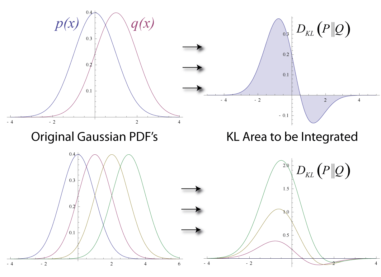
KL divergence (Kullback-Leibler57) or KL distance is non-symmetric measure of difference between two probability distributions. It is related to mutual information and can be used to measure the association between two random variables.

In this short tutorial, I show how to compute KL divergence and mutual information for two categorical variables, interpreted as discrete random variables.

${\bf Definition}$: Kullback-Leibler (KL) Distance on Discrete Distributions

Figure: Distance between two distributions. (Wikipedia)

Given two discrete probability distributions ${\it P}(A)$ and ${\it Q}(B)$ with discrete random variates, $A$ and $B$, having realisations $A=a_{j}$ and $B=b_{j}$, over $n$ singletons $j=1,...,n$. KL divergence or distance $D_{KL}$ in between $P$ and $Q$ is defined as follows:

$D_{KL} = D_{KL}\big({\it P}(A) || {\it Q}(B)\big)=\sum_{j=1}^{n} {\it P}(A=a_{j}) \log \Big(  \cfrac{{\it P}(A=a_{j})}{{\it Q}(B=b_{j})} \Big)$

$\log$ is in base $e$.

${\bf Definition}$: Mutual Information on Discrete Random Variates

Two discrete random variables $X$ and $Y$, having realisations $X=x_{k}$ and $Y=y_{l}$, over $m$ and $n$ singletons $k=1,...,n$ and $l=1,...,m$ respectively, are given. Mutual information, $I(X;Y)$ is defined as follows,

$I(X;Y) = \sum_{k=1}^{n} \sum_{l=1}^{m} {\it R}(X=x_{k}, Y=y_{l}) \log \Big(\cfrac{  {\it R}(X=x_{k}, Y=y_{l})  }{  {\it R}(X=x_{k})  {\it R}(Y=y_{l})} \Big)$

$\log$ is in base $e$ and $R$ denotes probabilities.

${\bf Definition}$: Mutual Information on Discrete Random Variates with KL distance

Two discrete random variables $X$ and $Y$. Mutual information, $I(X;Y)$ is defined as follows,

$I(X;Y) = D_{KL} \Big( {\it R}(X, Y) || {\it R}(X) {\it R}(Y) \Big)$

${\bf Problem: Example}$: Given two discrete random variables $X$ and $Y$ defined on the following sample spaces $(a,b,c)$ and $(d,e)$ respectively. Write down the expression for the mutual information, I(X;Y), expanding summation.

${\bf Solution: Example}$:

$I(X;Y)  = {\it R}(X=a, Y=d) \log \Big(\cfrac{ {\it R}(X=a, Y=d) }{  {\it R}(X=a)  {\it R}(Y=d)} \Big) +$

${\it R}(X=b, Y=d) \log \Big(\cfrac{  {\it R}(X=b, Y=d)  }{  {\it R}(X=b)  {\it R}(Y=d)} \Big)+$

${\it R}(X=c, Y=d) \log \Big(\cfrac{  {\it R}(X=c, Y=d)  }{  {\it R}(X=c)  {\it R}(Y=d)} \Big)+$

${\it R}(X=a, Y=e) \log \Big(\cfrac{  {\it R}(X=a, Y=e)  }{  {\it R}(X=a)  {\it R}(Y=e)} \Big)+$

${\it R}(X=b, Y=e) \log \Big(\cfrac{  {\it R}(X=b, Y=e)  }{  {\it R}(X=b)  {\it R}(Y=e)} \Big)+$

${\it R}(X=c, Y=e) \log \Big(\cfrac{  {\it R}(X=c, Y=e)  }{  {\it R}(X=c)  {\it R}(Y=e)} \Big)$


${\bf Definition}$: Two discrete random variables $X$ and $Y$, having realisations $X=x_{k}$ and $Y=y_{l}$, over $m$ and $n$ singletons $k=1,...,n$ and $l=1,...,m$ respectively, are given. Two-way contingency table of realisations of $X$ and $Y$ along the same measured data points, $N$ observations, can be constructed by counting co-occurances, or cross-classifying factors. Normalizing the resulting frequency table will produce joint and marginal probabilities.

                Y=y_{1}              ...    Y=y_{l}              R(X)
               
    X=x_{1}    R(X=x_{1}, Y=y_{1})   ... R(X=x_{1}, Y=y_{l}) R(X=x_{1})
    X=x_{2}    R(X=x_{2}, Y=y_{1})   ... R(X=x_{2}, Y=y_{l}) R(X=x_{2})
    ...             ...              ...        ...              ...
    X=x_{k}    R(X=x_{k}, Y=y_{1})   ... R(X=x_{k}, Y=y_{1} R(X=x_{k}) 
   
    R(Y)        R(Y=y{1})           ...  R(Y=y_{l})


Simulated example with R


 1
 2
 3
 4
 5
 6
 7
 8
 9
10
11
12
13
14
15
16
17
18
set.seed(3951824)
# Table of counts (contingency)
X <- sample(letters[1:3], 100, 1)
Y <- sample(letters[4:5], 100, 1)
t  <- table(X,Y)
tp  <- t/100 # proportions
tn  <- tp/sum(tp)     # normalized, joints
p_x <- rowSums(tn)    # marginals
p_y <- colSums(tn)

P <- tn 
Q <- p_x %o% p_y 

# P(X, Y)   : bin frequency: P_i
# P(X) P(Y) : bin frequency, Q_i 
mi <- sum(P*log(P/Q))
library(entropy)
mi.empirical(t) == mi

References

(KullbackLeibler57) Kullback, S.; Leibler, R.A. (1951). "On information and sufficiency". Annals of Mathematical Statistics 22 (1): 79–86. 


(c) Copyright 2008-2024 Mehmet Suzen (suzen at acm dot org)

Creative Commons License
This work is licensed under a Creative Commons Attribution 4.0 International License